ScholarWorks@UMass Amherst

Follow

• 

  Designing Sustainable Landscapes: Untransformed average annual daily traffic rate

  Kevin McGarigal, Brad Compton, Ethan Plunkett, Bill DeLuca, and Joanna Grand

• 

  Designing Sustainable Landscapes: HUC6 Watersheds

  Kevin McGarigal, Ethan Plunkett, Brad Compton, Bill DeLuca, and Joanna Grand

  This layer defines the subregions used for building cores in DSL landscape design (see technical document on landscape design, McGarigal et al 2017). It is based on the USGS Hydrologic Unit Codes (HUC) as extended in the USDA Watershed Boundary Dataset at the 6th level of the hierarchy (thus HUC6). In their original form these represent watersheds, sections of watersheds, and, especially in coastal areas, collections of watersheds of approximately equal size. They were chosen as the basic unit of our analysis because they were the size that stakeholders desired for subregions; are defined largely by natural boundaries, and are reasonably compact. We clipped the HUC6 boundaries to the Northeast Region and then manually edited the boundaries to make the HUCs and HUC fragments that remained within the Northeast Region more uniform in size and eliminate most disjunct HUC6s.

• 

  Designing Sustainable Landscapes: Climate Stress Metric

  Kevin McGarigal, Brad Compton, Ethan Plunkett, Bill DeLuca, and Joanna Grand

  Climate is a major factor in determining ecosystem distribution, composition, structure and function. Therefore, with climate change it is reasonable to anticipate heterogeneous climate stress across the landscape in response to heterogeneous shifts in climate normals (Iverson et al. 2014). The climate stress metric assesses the estimated climate stress that may be exerted on a focal cell in 2080 based on departure from the current climate niche breadth of the corresponding ecosystem. Essentially, this metric measures the magnitude of climate change stress at the focal cell based on the current climate niche of the corresponding ecosystem and the predicted change in climate (i.e., how much is the climate of the focal cell moving away from the current climate niche of the corresponding ecosystem) between 2010-2080 based on the average of two climate change scenarios (see below) (Fig. 1). Cells where the predicted climate suitability in the future decreases (i.e., climate is becoming less suitable for that ecosystem) are considered stressed, and the stress increases as the predicted climate becomes less suitable based on the ecosystem's current climate niche model. Conversely, cells where the predicted climate suitability in the future increases (i.e., climate is improving for that ecosystem) are considered unstressed and assigned a value of zero.

  The climate stress metric is an element of the ecological integrity analysis of the Designing Sustainable Landscapes (DSL) project (see technical document on integrity, McGarigal et al 2017). Consisting of a composite of 21 stressor and resiliency metrics, the index of ecological integrity (IEI) assesses the relative intactness and resiliency to environmental change of ecological systems throughout the northeast. As a stressor metric, climate stress values range from 0 (no effect from climate stress) to a theoretical maximum of 1 (severe effect; although in real landscapes, the metric never reaches 1). Note that the climate stress metric is computed separately for each ecosystem because each ecosystem has its own estimated climate niche (see below). This contrasts with all other stressor metrics, which are computed i

• 

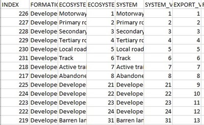
  Designing Sustainable Landscapes: DSLland and Subsysland

  Kevin McGarigal, Brad Compton, Ethan Plunkett, Bill DeLuca, and Joanna Grand

  DSLland is the land cover map used as an organizational framework in the Designing Sustainable Landscapes (DSL) project (McGarigal et al 2017). It is derived primarily from The Nature Conservancy's Northeast Habitat Classification

  map (Ferree and Anderson 2013; Anderson et al. 2013; Olivero and Anderson 2013; Olivero-Sheldon et al 2014). To meet the needs of the DSL project, we substantially modified the TNC map. The TNC map is a hierarchical classification. For our purposes, we adopted the 'habitat' level of the hierarchy, which we refer to as "ecosystems", as our finest scale, as it is the most appropriate classification for our ecological assessment. The attribute table also includes the ‘formation’ level for users that prefer a coarse classification.

• 

  Ecological integrity metrics: All integrity data products

  Kevin McGarigal, Brad Compton, Ethan B. Plunkett, Bill DeLuca, and Joanna Grand

  The ecological integrity products represent a set of metrics corresponding to our ecosystem-based ecological assessment in 2010 (see Integrity document for details). The ecological integrity metrics include a variety of measures of intactness and resiliency. The individual metrics are also combined into a composite local index of ecological integrity (IEI).

• 

  Designing Sustainable Landscapes: The index of ecological impact

  Kevin McGarigal, Brad Compton, Ethan Plunkett, Bill DeLuca, and Joanna Grand

  Includes five landscape change scenarios: 1) baseline 70-year (2010-2080) climate change and urban growth scenario without additional land protection; 2) same as #1 but with 25% more demand for new development; 3) same as #1 but with increased sprawl to the pattern of development; 4) same as #1 but with both 25% more demand for new development and increased sprawl; and 5) same as #1 but with additional terrestrial reserve areas (core areas) protected from development as established for Nature's Network landscape design (www.naturesnetwork.org).

• 

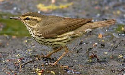
  Designing Sustainable Landscapes: Habitat loss, mowing and plowing, microclimate alterations, edge predators, domestic predators, invasive plants, and invasive earthworms metrics

  Kevin McGarigal, Brad Compton, Ethan Plunkett, Bill DeLuca, and Joanna Grand

  This document describes a suite of stressor metrics that assess different aspects of the effects of roads and development on ecological integrity (see technical document on integrity, McGarigal et al 2017). They share a common algorithm, but each has unique parameters. These metrics are obviously highly correlated, but each assesses a different aspect of the effects of roads and development on ecological integrity. These metrics are elements of the ecological integrity analysis of the Designing Sustainable Landscapes (DSL) project (McGarigal et al 2017). Consisting of a composite of 21 stressor and resiliency metrics, the index of ecological integrity (IEI) assesses the relative intactness and resiliency to environmental change of ecological systems throughout the northeast. These stressor metrics range from 0 (no effect) to 1 (severe effect). See Table 1 for parameters for each metric. Habitat loss. Assesses the intensity of past habitat loss caused by all forms of development. Direct habitat loss is the primary cause of species decline and extinction; this metric is an index of indirect habitat loss—the decline of integrity in remaining natural lands due to the loss of former habitat in the neighborhood to past development. Mowing and plowing. Assess the intensity of agriculture in the neighborhood as a surrogate for mowing and plowing rates, which are direct sources of animal mortality. Agricultural machinery is a well-known cause of mortality for grassland bird nestlings and terrestrial and semi-aquatic turtles. Microclimate alterations. Assesses microclimatic alterations due to edge effects, such decreased moisture, higher wind, and more extreme temperatures. This metric includes the effects of both anthropogenic edges and natural edges (e.g., the effects of an open marsh on the surrounding forest). Edge predators. Assesses the effect of human commensal mesopredators such as raccoons and skunks. Mesopredators often reach unusually high densities near human habitation, both due to food subsidies (garbage, bird feeders, and livestock grain) and mesopredator release. Domestic predators. Assesses the effect of domestic predators (primarily housecats) due to development. Both pet and feral housecats kill large numbers of birds and small mammals. Invasive plants. Assesses the effect of non-native invasive plants. Invasive plants often spread from sources in residential and agricultural areas, from humandisturbed areas, and along roads. Invasive earthworms. Assesses the effect of non-native invasive earthworms. In the glaciated northeast, all terrestrial earthworms are non-native. Spreading from agricultural areas, home gardens, and fishing holes, they speed up the nutrient cycle in nearby forests, often greatly affecting understory plants and seedling regeneration.

• 

  Designing Sustainable Landscapes: Index of Ecological Integrity

  Kevin McGarigal, Brad Compton, Ethan Plunkett, Bill DeLuca, and Joanna Grand

  The index of ecological integrity (IEI) is a measure of relative intactness (i.e., freedom from adverse human modifications and disturbance) and resiliency to environmental change (i.e., capacity to recover from or adapt to changing environmental conditions driven by human land use and climate change). It is a composite index derived from up to 21 different landscape metrics, each measuring a different aspect of intactness (e.g., road traffic intensity, percent impervious) and/or resiliency (e.g., ecological similarity, connectedness) and applied to each 30 m cell (see technical document on integrity, McGarigal et al 2017). The index is scaled 0-1 by ecological system and geographic area, such that it varies from sites with relatively low integrity (representing highly developed and/or fragmented areas) to relatively high integrity (representing large, undisturbed natural areas) within each ecosystem type and geographic area (e.g., Northeast, state, ecoregion, watershed). Consequently, boreal forests are compared to boreal forests and emergent marshes are compared to emergent marshes, and so on for each ecosystem type within the specified geographic extent. It doesn't make sense to compare the integrity of an average boreal forest cell to that of an average emergent marsh cell, because the latter have been substantially more impacted by human activities than the former. Scaling by ecological system means that all the cells within an ecological system are ranked against each other in order to determine the cells with the greatest relative integrity for each ecological system within the specified geographic extent.

• 

  Designing Sustainable Landscapes: Resiliency metrics: similarity, connectedness, and aquatic connectedness

  Kevin McGarigal, Brad Compton, Ethan Plunkett, Bill DeLuca, and Joanna Grand

  This document describes three resiliency metrics that measure a system’s ability to recover from disturbance or stress, as opposed to the other metrics, which assess sources of anthropogenic stress. Resiliency is both a function of the local ecological setting, since some settings are naturally more resilient to disturbance and stress (e.g., an isolated wetland is less resilient to species loss than a well-connected wetland because the latter has better opportunities for recolonization of constituent species), and the level of anthropogenic stress, since the greater the stressor the less likely the system will be able to fully recover or maintain ecological functions. All three of these metrics are based on assessing the distance from the focal cell to cells in its neighborhood in ecological settings space, as defined by a suite of 24 ecological settings variables. The settings variables are an attempt to capture the geophysical attributes that are primary determinants of ecological systems, e.g., temperature, sunlight, moisture, hydrology, and soils (McGarigal et al 2017). Settings also include several anthropogenic variables, such as development, traffic rates, and impervious surfaces. Ecological distance is low for points that fall nearby in settings space (e.g., two points that are on dry ridgetops with similar soils and climate), and higher for points that are further apart in settings space (e.g., a ridgetop and a valley wetland). Ecological distance is highest between natural and anthropogenic points (e.g., the ecological distance between a forest and a point in the middle of an expressway is extremely high, despite any similarities in landform or climate). Note that ecological distance is unrelated to physical distance (although two points that are nearby are more likely to share similar ecological settings).

• 

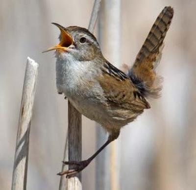
  Designing Sustainable Landscapes: Salt Marsh Ditching Metric

  Kevin McGarigal, Brad Compton, Ethan Plunkett, Bill DeLuca, and Joanna Grand

  The majority of salt marsh ditches in the Northeast have been ditched, both to facilitate harvest of salt marsh hay and to control mosquitoes (Smith and Niles 2016). Ditching changes the hydrology and flows of sediment and nutrients of marshes in ways that are not well understand, though ditched marshes may have altered invertebrate and shorebird communities, and may be less resilient to sea level rise (LeMay 2007). Marshes with intensive ditching (ca. 10 m spacing) appear to be most strongly affected (Vincent et al. 2013). The salt marsh ditching metric is an element of the ecological integrity analysis of the Designing Sustainable Landscapes (DSL) project (see technical document on integrity, McGarigal et al 2017). Consisting of a composite of 21 stressor and resiliency metrics, the index of ecological integrity (IEI) assesses the relative intactness and resiliency to environmental change of ecological systems throughout the northeast. As a stressor metric, salt marsh ditching provides an index of the relative intensity of ditching in salt marshes. Metric values range from 0 (no effect from nearby ditches) to 1 (severe effect). The metric is based on a custom image analysis process that identifies most ditches in salt marshes throughout the northeast from 1 m LiDAR (Light Detection And Ranging)-based DEMs (Digital Elevation Models). The algorithm, uses a kernel to identify local depressions that could be ditches. It then uses a morphological skeletonize algorithm to draw a 1 m-wide line through the middle of depressions, and then uses an original approach, “clockfacing,” to find linear features in these centerlines of depressions and connect disconnected sections. These potential ditches are converted from raster to linear features, and long, fairly straight sections are tagged as ditches. These linear ditches are converted back to a 1 m raster, then to a 30 m raster, with a value indicating ditch density in each cell. Finally, the ditching metric itself measures the intensity of ditches in the neighborhood of each salt marsh cell using a kernel estimator. Funding for this project was provided by the North Atlantic Landscape Conservation Cooperative and Department of the Interior Project #24, Decision Support for Hurricane Sandy Restoration and Future Conservation to Increase Resiliency of Tidal Wetland Habitats and Species in the Face of Storms and Sea Level Rise.

• 

  Designing Sustainable Landscapes: Sea level rise metric

  Kevin McGarigal, Brad Compton, Ethan Plunkett, Bill DeLuca, and Joanna Grand

  The sea level rise metric estimates the probability of the focal cell being unable to adapt to predicted inundation by sea level rise (SLR). Whether a site gets inundated by salt water permanently due to sea level rise or intermittently via storm surges associated with sea level rise determines whether an ecosystem can persist at a site and thus its ability to support a characteristic plant and animal community. Based on a sea level rise inundation model developed by USGS Woods Hole (Lentz et al. 2015). The sea level rise metric is an element of the ecological integrity analysis of the Designing Sustainable Landscapes (DSL) project (see technical document on integrity, McGarigal et al 2017). Consisting of a composite of 21 stressor and resiliency metrics, the index of ecological integrity (IEI) assesses the relative intactness and resiliency to environmental change of ecological systems throughout the northeast. As a stressor metric, sea level rise ranges from 0 (no effect from sea level rise) to 1 (severe effect). Sea level rise is only applied to future time steps; for 2010, the value of sea level rise is always zero.

• 

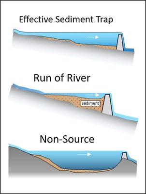
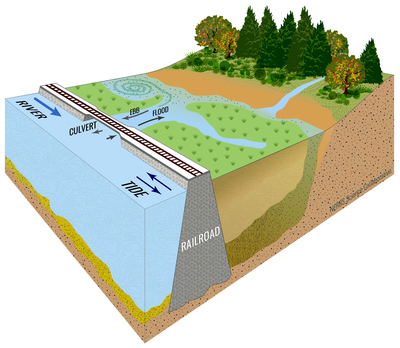
  Designing Sustainable Landscapes: Tidal Restrictions metric

  Kevin McGarigal, Brad Compton, Ethan Plunkett, Bill DeLuca, and Joanna Grand

  Tidal restrictions include undersized culverts and bridges, tide gates, dikes, and other structures that interfere with normal tidal flushing in estuarine systems. Effects can range from mild changes in species composition and cycling of sediment and nutrients to wholesale conversion of ecological systems, such as conversion of Spartina-dominated salt marshes to Phragmites australis, or, in extreme cases, to freshwater wetlands (Roman et al. 1984, Ritter et al. 2008). The tidal restrictions metric is an element of the ecological integrity analysis of the Designing Sustainable Landscapes (DSL) project (see technical document on integrity, McGarigal et al 2017). Consisting of a composite of 21 stressor and resiliency metrics, the index of ecological integrity (IEI) assesses the relative intactness and resiliency to environmental change of ecological systems throughout the northeast. As a stressor metric, tidal restrictions uses an estimate of the historic loss of mapped salt marshes in areas where they should occur given elevation and tidal regime to indicate the location and magnitude of potential tidal restrictions. The metric estimates the effect of potential tidal restrictions on upstream wetland systems, including intertidal systems such as salt marshes, as well as freshwater systems and low-lying nonforested uplands that may have once been intertidal. Metric values range from 0 (no effect from downstream tidal restrictions) to 1 (severe effect). The metric is based on an estimate of the salt marsh loss ratio above each potential tidal restriction (road-stream and railroad-stream crossings). Note that tide gates not associated with roads are excluded as potential tidal restrictions, as they are not comprehensively mapped throughout the region. The salt marsh loss ratio is the proportion of a basin above a crossing that is modeled as potential salt marsh (from tide range and elevation) but not mapped as existing salt marsh in the National Wetlands Inventory (NWI) maps. Funding for this project was provided by the North Atlantic Landscape Conservation Cooperative and Department of the Interior Project #24, Decision Support for Hurricane Sandy Restoration and Future Conservation to Increase Resiliency of Tidal Wetland Habitats and Species in the Face of Storms and Sea Level Rise.

• 

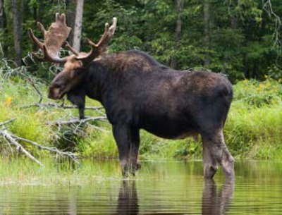
  Designing Sustainable Landscapes: Traffic metric

  Kevin McGarigal, Brad Compton, Ethan Plunkett, Bill DeLuca, and Joanna Grand

  The traffic metric assesses the effect of road (and railroad) traffic on animal populations due to road mortality. It integrates the distance to and traffic intensity of roads in the neighborhood of the focal cell. The traffic metric (Fig. 1) is an element of the ecological integrity analysis of the Designing Sustainable Landscapes (DSL) project (see technical document on integrity, McGarigal et al 2017). Consisting of a composite of 21 stressor and resiliency metrics, the index of ecological integrity (IEI) assesses the relative intactness and resiliency to environmental change of ecological systems throughout the northeast. As a stressor metric, Traffic values range from 0 (no effect from road traffic) to 1 (severe effect; although in real landscapes, the metric never reaches 1).

• 

  Designing Sustainable Landscapes: Wind exposure settings variable

  Kevin McGarigal, Brad Compton, Ethan Plunkett, Bill DeLuca, and Joanna Grand

  Wind exposure is one of several ecological settings variables that collectively characterize the biophysical setting of each 30 m cell at a given point in time (McGarigal et al 2017). Wind exposure gives the mean sustained wind speed (m/s) at 50 m height. High wind speeds can shape natural communities, especially on exposed high peaks.

• 

  Designing Sustainable Landscapes: Watershed habitat loss, watershed imperviousness, road salt, sediment, nutrients, and dam intensity metrics

  Kevin McGarigal, Brad Compton, Ethan Plunkett, Bill DeLuca, and Joanna Grand

  This document describes a suite of stressor metrics that assess the various effects of development in the watershed of the focal cell, as opposed to a (usually) circular window around the focal cell, as with the other metrics. These metrics are used for lotic, lentic, and wetland systems. All effects are weighted by a the time of flow from each stressor source to the focal cell, thus, stressor sources that fall within a stream have a greater effect than those in distant uplands within the watershed. These share a common algorithm, but each has unique parameters. These metrics are elements of the ecological integrity analysis of the Designing Sustainable Landscapes (DSL) project (see technical document on integrity, McGarigal et al 2014). Consisting of a composite of 21 stressor and resiliency metrics, the index of ecological integrity (IEI) assesses the relative intactness and resiliency to environmental change of ecological systems throughout the northeast. These stressor metrics range from 0 (no effect) to maximum values that differ for each metric (severe effect). See Table 1 for parameters for each metric.

• 

  Designing Sustainable Landscapes: Water salinity settings variable

  Kevin McGarigal, Brad Compton, Ethan Plunkett, Bill DeLuca, and Joanna Grand

  Water salinity is one of several ecological settings variables that collectively characterize the biophysical setting of each 30 m cell at a given point in time (McGarigal et al 2017). Salinity, which varies from 0‰ in freshwater to 30‰ in seawater, is a major driver of aquatic systems, as very few organisms can survive across this full range.

• 

  Designing Sustainable Landscapes: Topographic wetness and Flow volume settings variables

  Kevin McGarigal, Brad Compton, Ethan Plunkett, Bill DeLuca, and Joanna Grand

  Topographic wetness and flow volume are two of several ecological settings variables that collectively characterize the biophysical setting of each 30 m cell at a given point in time (McGarigal et al 2017). These variables are two ways of assessing the flow of water; they share an underlying algorithm. Topographic wetness gives an estimate of the amount of moisture at any point in the landscape based on topography, which has a major effect on species habitat, soils, and the nutrient cycle. It ranges, in arbitrary units, from low values at hilltops and steep upper slopes to high values in low, flat areas with high flow accumulation. All lotic and lentic waterbodies share the same maximum value. Flow volume ranges in arbitrary units from 0 in uplands to a maximum in large rivers. It estimates the amount of water flowing into and through aquatic and wetland systems, which, along with gradient, largely determines species habitat and sediment transport. Flow volume is often coarsely estimated by stream order.

• 

  Designing Sustainable Landscapes: Tides settings variable

  Kevin McGarigal, Brad Compton, Ethan B. Plunkett, Bill DeLuca, and Joanna Grand

  Tides is one of several ecological settings variables that collectively characterize the biophysical setting of each 30 m cell at a given point in time (McGarigal et al 2017). Tides estimates the probability that a point is intertidal or subtidal. It is derived from a logistic regression model using tide range and elevation to distinguish mapped salt marshes from uplands.

• 

  Designing Sustainable Landscapes: Terrestrial barriers settings variable

  Kevin McGarigal, Brad Compton, Ethan B. Plunkett, Bill DeLuca, and Joanna Grand

  Terrestrial barriers is one of several ecological settings variables that collectively characterize the biophysical setting of each 30 m cell at a given point in time (McGarigal et al 2017). Terrestrial barriers measures the relative degree to which roads and railroads may physically impede movement of terrestrial organisms. It is derived by assigning an expertderived score to each road/railroad class to reflect the increasing physical impediment of larger roads, and adjusting these scores at road-stream crossings (i.e., bridge or culvert) based either on a custom algorithm applied to field measurements of the crossing structure or predictions from a statistical model (see below for details) to reflect increased passability of terrestrial organisms through the crossing structure. Terrestrial barriers is scaled 0-5, where roads and railroads are assigned values >0 (indicating the relative degree of impediment) and all other cells are assigned 0.

• 

  Designing Sustainable Landscapes: Substrate mobility settings variable

  Kevin McGarigal, Brad Compton, Ethan B. Plunkett, Bill DeLuca, and Joanna Grand

  Substrate mobility is one of several ecological settings variables that collectively characterize the biophysical setting of each 30 m cell at a given point in time (McGarigal et al 2017). Substrate mobility measures the realized mobility of the physical substrate, due to both substrate composition (e.g., sand) and exposure to forces (wind and water) that transport material. This is an important attribute of certain dynamic systems (e.g., coastal dune systems); given as a simple index of mobility (1 = stable, 10 = highly mobile). Substrate mobility is assigned by landcover class, derived from expert opinion. This settings variable is dynamic, changing with urban growth.

• 

  Designing Sustainable Landscapes: Stream temperature settings variable

  Kevin McGarigal, Brad Compton, Ethan Plunkett, Bill DeLuca, and Joanna Grand

  Stream temperature is one of several ecological settings variables that collectively characterize the biophysical setting of each 30 m cell at a given point in time (McGarigal et al 2017). Several fish species (e.g., brook trout) can only survive in coldwater streams, which have higher levels of dissolved O2, while other fish species are adapted to warmer streams. At the same time, ectotherms such as aquatic insects and fish can develop more quickly in warmer streams. Stream temperature is a coarse classification of streams by mean annual temperature.

• 

  Designing Sustainable Landscapes: Soil available water supply, Soil depth to restrictive layer, and Soil pH settings variables

  Kevin McGarigal, Brad Compton, Ethan Plunkett, Bill DeLuca, and Joanna Grand

  These three soils variables are among several ecological settings variables that collectively characterize the biophysical setting of each 30 m cell at a given point in time (McGarigal et al 2017). Soils are important drivers of natural communities. We picked three soil attributes that represent the most important factors: depth, chemistry, and water-holding capacity. Depth to resistant layer measures the depth of soils to a restrictive layer (e.g., bedrock) that limits root depth. Areas with shallow soils (usually on steep slopes or ridgetops) can’t support deep-rooted plants. Soil pH strongly affects nutrient uptake by plants. In the east, soils with higher pH (e.g., in areas with limestone bedrock) tend to support a greater diversity of plants, including a number of species that typically grow only in sweet soils. Conversely, some groups of plants (such as members of Ericaceae) are specialized to acidic soils, where generalist species grow poorly at best. Available water supply (AWS) measures the water-holding capacity of soils. It is measured as the total volume of water that available to plants when the soil, inclusive of rock fragments, is at field capacity. Soils with a high AWS are more drought-resistant, supporting plant growth through periods without rain—for instance, good agricultural soils have a high AWS. AWS is calculated as the available water capacity times the thickness of each soil horizon to a specified depth (25 cm in this case). Note that AWS is distinct from our topographic wetness settings variable, which estimates the amount of water delivered to the soil at each point.

• 

  Designing Sustainable Landscapes: Slope settings variable

  Kevin McGarigal, Brad Compton, Ethan Plunkett, Bill DeLuca, and Joanna Grand

  Slope is one of several ecological settings variables that collectively characterize the biophysical setting of each 30 m cell at a given point in time (McGarigal et al 2017). Slope gives the percent slope at each cell. High slopes indicate a propensity for gravityinduced physical disturbance (e.g., talus slopes), which can limit plant development. Slope ranges from 0% for flat areas to theoretically infinity for absolutely vertical cliffs, though the actual maximum occurring in our landscape is 440%.

• 

  Designing Sustainable Landscapes: Potential dominant life form settings variable

  Kevin McGarigal, Brad Compton, Ethan Plunkett, Bill DeLuca, and Joanna Grand

  Potential dominant life form is one of several ecological settings variables that collectively characterize the biophysical setting of each 30 m cell at a given point in time (McGarigal et al 2017). Potential dominant life form (unvegetated, herbaceous, shrubland, woodland, forest) represents the structure of vegetative community at a site and is used, for example, to distinguish early successional forest from permanent grassland or shrubland. Potential dominant life form is assigned by landcover class, derived from expert opinion. This settings variable is dynamic, changing with urban growth.

• 

  Designing Sustainable Landscapes: Imperviousness settings variable

  Kevin McGarigal, Brad Compton, Ethan Plunkett, Bill DeLuca, and Joanna Grand

  Imperviousness is one of several ecological settings variables that collectively characterize the biophysical setting of each 30 m cell at a given point in time (McGarigal et al 2017). Imperviousness measures the percentage of the ground surface area that is impervious to water infiltration, which is an indicator of intensive development and thus an important determinant of ecological communities. This is a dynamic settings variable, increasing with future urban growth.